Excel

Formulas

Every formula has the following 3 parts:

= Function Name (Arguments)

Evaluate Formulas: This is a great tool to debug formulas. It’s similar to code debugging where you can step in to a formula and see at each step what a formula returns. This can be found at Formulas > Formula Auditing > Evaluate Formulas.

• Excel functions (alphabetical)
• Excel functions (by category)

Common Functions

Function	Description	Example
SUM(number1, [number2], …)	Calculates the sum of a group of values.	=SUM(A2:A10)
MAX(number1, [number2], …)	Returns the largest value in a set of values.	=MAX(A2:A10)
MIN(number1, [number2], …)	Returns the smallest number in a set of values.	=MIN(A2:A10)
AVERAGE(number1, [number2], …)	Calculates the mean of a group of values.	=AVERAGE(A2:A10)
COUNT(value1, [value2], …)	Counts the number of cells in a range that contains numbers.	=COUNT(A2:A10)
COUNTA(value1, [value2], …)	Counts the number of cells that are not empty in a range.	=COUNTA(A2:A10)

Math Functions

Function	Description	Example
INT(number)	Rounds a number down to the nearest integer.	=INT(A2)
ROUND(number, num_digits)	Rounds a number to a specified number of digits.	=ROUND(2.15, 1)
ROUNDDOWN(number, num_digits)	Rounds a number down, toward zero.	=ROUNDDOWN(3.2, 0)
ROUNDUP(number, num_digits)	Rounds a number up, away from 0 (zero).	=ROUNDUP(3.2,0)
SUBTOTAL(function_num,ref1,[ref2],…)	Returns a subtotal in a list or database. It is generally easier to create a list with subtotals by using the Subtotal command in the Outline group on the Data tab in Excel.	=SUBTOTAL(1,A2:A5)
SUMIF(range, criteria, [sum_range])	Adds the cells specified by a given criteria	=SUMIF(A2:A5,">160000",B2:B5)

IF() Function

Explain function. Maybe use table above.

=IF(F5>=Goal,"YES","NO")

AND Function

COUNTIF()

SUMIF()

VLOOKUP(): Look up values in another worksheet vertically. This is often helpful if you are trying to pull exact values from one worksheet to another.

Examples:

=VLOOKUP($B3,'Master Emp List'!$A$1:$I$38,2,FALSE)

VLOOKUP() parameters:

• Lookup_value: Typically the ID to reference another table.
• Table_array: The entire table that you are referencing in another worksheet. The lookup_value must be the found in the first column of this table.
• Col_index_num: The column number that you want to pull from the other worksheet. This is base 1.
• Range_lookup: If you want an exact match use “FALSE”, otherwise use “TRUE”. Most often we’ll use FALSE.

HLOOKUP(): Look up values in another worksheet horizontally. This follows the same format as VLOOKUP(), but is just horizontal.

INDEX(): Returns a value at a specific position in a list. You provide the cells to search, then the row and column number (e.g. 4). This pinpoints an exact match in the spreadsheet. This most likely will not be used often on its own.

MATCH(): Returns a numeric position of a value. It’s the opposite of INDEX() where you provide a value, and it tells you which field it’s in.

Errors

Error	Explanation
#DIV/0!	Trying to divide by 0.
#VALUE!	There’s something wrong with the way your formula is typed. Or, there’s something wrong with the cells you are referencing. The error is very general, and it can be hard to find the exact cause of it. Troubleshoot
#NUM!	A formula or function contains numeric values that aren’t valid. Troubleshoot
#N/A	A formula or a function inside a formula cannot find the referenced data. Troubleshoot
#REF!	A formula refers to a cell that’s not valid. This happens most often when cells that were referenced by formulas get deleted, or pasted over. Troubleshoot
#NAME?	Text in the formula is not recognized. The top reason why the #NAME? error appears in your formula is because there is a typo in the formula name. Troubleshoot
#####	Excel might show ##### in cells when a column isn’t wide enough to show all of the cell contents. Formulas that return dates and times as negative values can also show as #####. Troubleshoot
#NULL!	A space was used in formulas that reference multiple ranges; a comma separates range references.

Shortcuts

For the most up to date shortcuts, refer to Microsoft’s help article. This table will list out shortcuts that I find useful.

Functionality	Shortcut
AutoSum	Alt + =
Select the column	Ctrl + Spacebar
Select the row	Shift + Spacebar
Add new row or column	Ctrl + Shift + Plus Sign (+)
Remove a row or column	Crtl + -
Highlight all cells above the currently selected cell	Ctrl + Shift + Up
Highlight all cells below the currently selected cell	Ctrl + Shift + Down
Highlight all cells to the right of the currently selected cell	Ctrl + Shift + Right
Highlight all cells to the left of the currently selected cell	Ctrl + Shift + Left

References

There are two types of cell references: relative and absolute.

1. Relative references change when a formula is copied to another cell.
2. Absolute references remain constant no matter where they are copied.

Relative References

By default, all cell references are relative references. When copied across multiple cells, they change based on the relative position of rows and columns.

For example, if you copy the formula =A1+B1 from row 1 to row 2, the formula will become =A2+B2. Relative references are especially convenient whenever you need to repeat the same calculation across multiple rows or columns.

Absolute Reference

There may be times when you do not want a cell reference to change when filling cells. Unlike relative references, absolute references do not change when copied or filled. You can use an absolute reference to keep a row and/or column constant.

Reference	Description
$A$2	The column and the row do not change when copied.
A$2	The row does not change when copied.
$A2	The column does not change when copied.

See Also:

• GCF Learn Free Relative and Absolute Cell References

Cell References with Multiple Worksheets

Excel allows you to refer to any cell on any worksheet, which can be especially helpful if you want to reference a specific value from one worksheet to another. To do this, you’ll simply need to begin the cell reference with the worksheet name followed by an exclamation point (!).

For example, if you wanted to reference cell A1 on Sheet1, its cell reference would be Sheet1!A1.

Note that if a worksheet name contains a space, you’ll need to include single quotation marks (‘ ‘) around the name. For example, if you wanted to reference cell A1 on a worksheet named July Budget, its cell reference would be 'July Budget'!A1.

Conditional Formatting

1. Highlight the cells.
2. Home > Styles > Conditional Formatting

Data Visualization

Pie charts are good for a single column or row.

Custom Sorts

If you have a column with the month spelled out, if you sort it ASC it will make it alphabetical. Excel has a built-in way to support sorting on the actual month values though.

1. Go to Data > Sort & Filter > Sort
2. Under Order click on “Custom List…”
3. Select the custom list.
4. Select the applicable list.

Subtotal

The Subtotal command allows you to automatically create groups and use common functions like SUM, COUNT, and AVERAGE to help summarize your data. For example, the Subtotal command could help to calculate the cost of office supplies by type from a large inventory order. It will create a hierarchy of groups, known as an outline, to help organize your worksheet.

https://edu.gcfglobal.org/en/excel2016/groups-and-subtotals/1/

Go to Data > Subtotal.

Duplicates

Select cells. Go to Conditional Formatting, highlight duplicates.

If the list is a table, under the Design tab there is a Remove Duplicates button under Tools.

Or Data > Remove Duplicates

DSUM

Sum up the total sales, but only where a category is equal to something.

Summing up a set of cells based on criteria. Database Sum.

DSUBTOTAL

If you have a table of data, it will displays accurately if the list is sorted.

PivotTable

A PivotTable allows you to extract the significance from a large, detailed data set.

Insert a PivotTable

1. Click any single cell inside the data set.
2. Go to Insert > Tables > PivotTable.

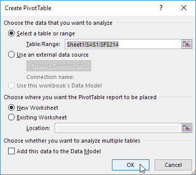
1. The following dialog box appears. Excel automatically selects the data for you. The default location for a new pivot table is New Worksheet.

Drag Fields

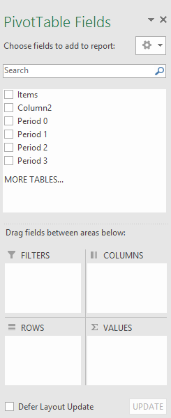
To add a field to your PivotTable, select the field name checkbox in the PivotTables Fields pane.

To move a field from one area to another, drag the field to the target area.

Drill Down

Within a PivotTable, if you double click on any cell, it will create a new worksheet with more details about how that cell is calculated.

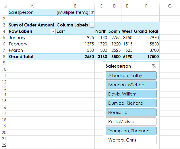
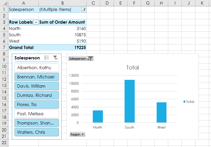
Slicers

Slicers make filtering data in PivotTables even easier. Slicers are basically just filters, but they’re easier and faster to use, allowing you to instantly pivot your data. If you frequently filter your PivotTables, you may want to consider using slicers instead of filters.

1. Select any cell in the PivotTable.
2. From the Analyze tab, click the Insert Slicer command.
3. A dialog box will appear. Select the desired field.
4. The slicer will appear next to the PivotTable.

PivotCharts

PivotCharts are like regular charts, except they display data from a PivotTable. Just like regular charts, you’ll be able to select a chart type, layout, and style that will best represent the data.

1. Select any cell in your PivotTable.
2. From the Insert tab, click the PivotChart command.
3. The Insert Chart dialog box will appear. Select the desired chart type and layout, then click OK.
4. The PivotChart will appear.

See Also:

• GCF Learn Free Excel - Intro to PivotTables
• Create a PivotTable to analyze worksheet data

Power Pivot

Power Pivot is a data modeling technology that lets you create data models, establish relationships, and create calculations. With Power Pivot you can work with large data sets, build extensive relationships, and create complex (or simple) calculations, all in a high-performance environment.

Enabling Power Pivot

Power Pivot must be enabled in Excel to be able to use it.

1. Go to File > Options > Add-Ins.
2. In the Manage box, click COM Add-ins> Go.
3. Check the Microsoft Office Power Pivot box, and then click OK.

Getting Started with Power Pivot

When the Power Pivot add-on is enabled, the Power Pivot tab in the ribbon is available, as shown in the following image.

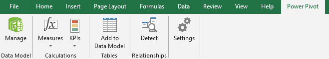
From the Power Pivot ribbon tab, select Manage from the Data Model section.

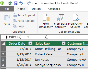
When you select Manage, the Power Pivot window appears, which is where you can view and manage the data model, add calculations, establish relationships, and see elements of your Power Pivot data model. A data model is a collection of tables or other data, often with established relationships among them. The following image shows the Power Pivot window with a table displayed.

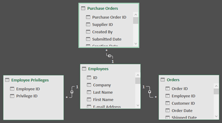
The Power Pivot window can also establish, and graphically represent, relationships between the data included in the model. By selecting the Diagram view icon from the bottom right side of the Power Pivot window, you can see the existing relationships in the Power Pivot data model. The following image shows the Power Pivot window in Diagram view.

With a Power Pivot, you can create a PivotTable that uses multiple worksheets.

See Also:

• Power Pivot Overview and Learning
• Create a Data Model in Excel
• Key Performance Indicators in Power Pivot

Name Manager

You can create variables with the textbox to the left of the formula bar.

Protecting Worksheets

Once you’ve made changes to a worksheet, you want to prevent people from changing things, such as formulas.

Protecting Specific Cells

Every cell has a locked property, and by default it is turned On.

You need to remove the Lock from cells, then protect it.

1. Select the cells you want people to be able to change.
2. Go to Home > Font > Font Settings > Protection.
3. Uncheck the Locked property.
4. Go to Review > Protect Sheet. Enter a password, select the options, hit enter.

Protecting the Structure of a Workbook

If a worksheet references another worksheet, we want to protect it so those references don’t get destroyed.

1. Go to Review > Changes > Protect Workbook
2. Enter in a password if desired. Click OK.

Protecting Workbooks prevent people from renaming worksheets, inserting, deleting, moving, etc.

What-If Analysis

Goal Seek

Pretty cool.

LEFT(): Get the set number of left characters.

=LEFT(A4,3)

RIGHT(): =RIGHT(A4,2)

MID(): Get characters in the middle of the cell.

=MID(A4,4,6)

LEN(): Returns the number of characters in a cell.

=LEN(A3)

SEARCH(): Search a string for a specific character.

SEARCH(A2)

To split on a Full Name field:

Full Name: Joe Burns.

• Get first name: =LEFT(A2,SEARCH(" ",A2))
• Get last name: =RIGHT(A2,LEN(A2)-SEARCH(" ",A2))

To concatenate individual names to a singular name:

Last Name	First Name
Smith	Howard

=CONCATENATE(B2," ",A2)

Auditing Worksheets

All of these items can be found in Formulas > Formula Auditing.

• Trace Precedents: This is pretty cool. It displays lines of cells that were used in the formula.
• Trace Dependents: Running this while in a cell will show what cells reference this cell.
• Watch Window: Mark a cell you want to watch to alert you if its value gets updated.
• Show Formulas: Displays the formulas right in the worksheet rather than the values. It’s helpful to review the worksheet and make sure the formulas are correct.

Macros

Macros allow you to automate tasks in Excel with code.

First you need to turn on the Developer tab.

1. Right click anywhere on the ribbon, and then click Customize the Ribbon.
2. Under Customize the Ribbon, on the right side of the dialog box, select Main tabs (if necessary).
3. Check the Developer check box.